|
Time
continuum: by quantum time evolution.
Continuum time, by continuum energetic hyper- space activity appears by
endless [evolution] of vortices [quanta] formations.
Time like Schrödinger cats paradox,alive
and not alive for ever.
Chaim, Henry Tejman Dr.
Emeritus,
Jerusalem university.
United
Nature-Wave theory
Tejman:
Continuum time: Constant active sophisticated energetic hyperspace composed
by three sophisticated constant active media:
Space, time and energy are waved together.
Each has its own properties and behaviours; one cannot exist
without the others. Theoretically, each of them has no beginning and no
end, and they are all one entity but are changeable, depending on different
phases of energetic matter in which they appear and decay together.
These
three media - time, space and energy create sophisticated regional vortex
wave-quantum creation with all energetic space time forces. Quantum formation
has beginning and end but by energetic space time [time quantum genes] create endless recrudescent quantum time [evolution]
future quanta of continue times.
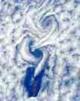
Continuum time and hyperspace by continuum vortices [quanta]
creation. A.
Einstein: Continue time: A four-dimensional continuum with four
coordinates, the three dimensions of space and that of time, in which any
event can be located.
United Nature
[Tejman] Continue time [Einstein]: A four-dimensional continuum with
four coordinates, the three dimensions of space and that of time, in which
any event can be located mainly by continuum endless evolution of quantum
creation.
In Newton's absolute universe, time as well as energetic
matter and space have neither a beginning nor an end as a main dimension.
On the other hand, Einstein's relative time does contain a beginning and end
together with the appearance of a formation and disperse, again to
the universe's, (to main dimensions) to form new energetic formations
(relative time time evolution). Absolute time cannot exist
without relative time and vice versa. Newton's absolute time is allied to
universal dimension and Einstein's time (relative time) is allied to
energetic matter quanta formations.
Time, as space and energy is a dimension of
the universe.
Without energetic activity space and time would not exist.
Quantum creation: Condensation
of energetic space time [Einstein] of regional swirl-circular vicious-vortex
creation [Tejman].
Quantum 3 D M-bubble, M.
Planck,
curled formation by regional
space time swirl .
Max Plank: quantum
constant [equilibrium of energetic forces]. creation
of everything.
|
|

|
|
|
Black hole radiation
|
Energetic-electric part of quantum symmetry
|
Magnetic-gravity part of quantum symmetry
|
|
|
|
|
|
|
Quantum-Gravitational
wave 3
D strings
[ of all quanta formations]-Space time geometry- bubble - A. Einstein,
Albert Einsteins
space time curvatures-is equation of quantum
|
|

|

|

|
|
|
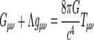
Einsteins equation 3D
|
|
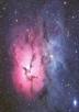
Visual Einsteins and Tejmans
quantum space time curvatures 3D
|
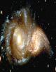
Galaxy two semi loops 3D quantum
|
|
|
|
|
|
|
|
A.
Einstein equation describe the relation between the geometry of a
four-dimensional, semi-Riemannian
manifold representing spacetime on the
one hand, and the energy-momentum contained
in that space time on the other. That is exactly quantum formation. creation
of everything Theory of everything, Einstein did that! But not imaginate
visually the quantum as appear in nature and United Nature theory by
introduction two behavior and phase transition of every quantum formation
[include living formations] explain this ingenious equation as the quantum
really appears in nature .
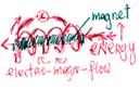
Quantum C.Tejman:
Composed by 3
D bubble strings energetic paths, which by
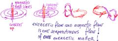
swirling rotation and revolving motion create strings wave formation of electro-magnetic and gravity
semi loops720 two perpendicular spins forces] two
semi perpendicular loops of gravitational
wave as really that appears in nature. The first laboratory quantum formation create
M. Faraday, with two main
perpendicular forces, exactly as Einsteins
and Tejman equations.
Faradays experiment.
Other
important quantum equations. 
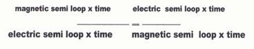
This Tejmans equation explain the behavior of the two
semi loops in photon phase transition.In different phase transitions the
proportion are other.
Every quantum creation composed by two main behaviors:
electric and magnetic-gravity.
|
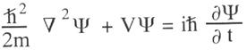
Schrödingers
equation:
|
|
|
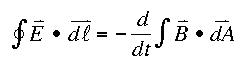
Faradays equation:
|
|
|
Maxwell equation:
|

|
|
Plancks
equation:
|

|
|
Einsteins
equation:
|

|
The de Broglie equation f =E/h, or E= fXh
TIME: appears together
with strings regional swirl vortex- quantum creation [the 4th dimension of
quantum],
by space time curvature, which by revolving and rotation motion create main electro-magnetic
force. Time continuum by space time curvature, with all forces obeys all
rules of quantum formation. There is not chaos. Everything [like in army]
obeys the hierarchy order by continuum time strings-energetic path from basic
main energetic swirl and its main electromagnetic force. Time vanishes
together with quantum disintegration [dispersion] and by evolution by quanta genes continue to form new future
quanta with all formations of inquired times.
Equation of everything
[Tejman]: Equilibrium of all energetic forces-times of quantum formation in all
different phase transitions.
Cit. CONTENTS · BIBLIOGRAPHIC RECORD http://www.bartleby.com/173/26.html
Albert Einstein (18791955). Relativity:
The Special and General Theory. 1920.
The Space-Time Continuum
of the Special Theory of Relativity Considered as a Euclidean Continuum
Minkowski found that the Lorentz transformations satisfy
the following simple conditions. Let us consider two neighbouring events, the
relative position of which in the four-dimensional continuum is given with
respect to a Galileian reference-body K by the space co-ordinate
differences dx, dy, dz and the time-difference dt. With
reference to a second Galileian system we shall suppose that the
corresponding differences for these two events are dx', dy', dz', dt'.
Then these magnitudes always fulfil the condition. 1

The
validity of the Lorentz transformation follows from this condition. We can
express this as follows: The magnitude ds2=dx2+dy2+dz2-c2dt2
which belongs to two adjacent points of the four-dimensional space-time
continuum, has the same value for all selected (Galilean) reference-bodies.
If we replace x, y, z, 
ds2=dx2+dy2+dz2-c2dt2
ds2=dx2+dy2+dz2-c2dt2
\
http://www.bartleby.com/173/26.html
Tejman: United
Nature-Wave theory
Infinite continue hyperspace by continue evolution of
quanta time [regional vortices] swirls.
Time Continuum: recurrence of quanta formations [time genes] as Continue
time [Einstein]: A four-dimensional continuum with four coordinates, the
three dimensions of space and that of time, in which any event can be located
mainly by continuum endless evolution of quantum creation.
|
Energetic semi loop
Time: Continuum
= ─────────
Quantum evolution.
Magnetic
semi loop
|
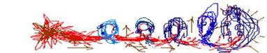
Time continuum: by motion of quanta
[vortex, swirl] by two perpendicular forces [two semi continuum
swirls]-electric and magnetic by four Einsteins four-dimensional
continuum with four coordinates.
In sophisticated energetic hyper-space
by continuum space time curvatures [A. Einstein] which by swirling rotation
and revolving motion create two perpendicular forces electro-magnetic that
create time quantum [everything].
In sophisticate
hyperspace, appears endless different vortices-quanta [endless wave frequency]
with their relative endless continuum times.
 wave frequency hence
constant wave frequency hence
constant

Other works:
http://en.wikipedia.org/wiki/Space-time_continuum
Spacetime intervals
 (spacetime interval), (spacetime interval),
Time-like interval
The measure of a time-like spacetime interval is described by
the proper time:
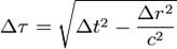 (proper time). (proper time).
Light-like interval
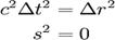
Space-like interval
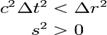
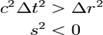
For these space-like event pairs with a positive squared
spacetime interval (s2 > 0), the
measurement of space-like separation is the proper distance:
 (proper distance). (proper distance).
Like the proper time of time-like intervals, the proper distance
(Δσ) of
space-like spacetime intervals is a real number value.
Spacetime
in special relativity Main
article: Minkowski
space The geometry of spacetime in special relativity is
described by the Minkowski metric on R4.
This spacetime is called Minkowski space. The Minkowski metric is usually
denoted by η and can be
written as a four-by-four matrix:
  Two-dimensional
analogy of spacetime distortion. Matter changes the geometry of spacetime,
this (curved) geometry being interpreted as gravity. White lines do
not represent the curvature of space but instead represent the coordinate
system imposed on
the curved spacetime, which would berectilinear in a flat spacetime. Two-dimensional
analogy of spacetime distortion. Matter changes the geometry of spacetime,
this (curved) geometry being interpreted as gravity. White lines do
not represent the curvature of space but instead represent the coordinate
system imposed on
the curved spacetime, which would berectilinear in a flat spacetime.

Other sources:
Mathematical
modeling of a continuum
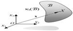
Figure 1. Configuration of a
continuum body 
Kinematics:
deformation and motion
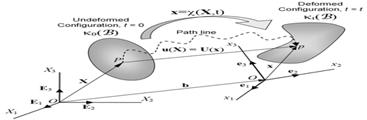
Figure
2. Motion of a continuum body.
The
material points forming a closed surface at any instant will always form a
closed surface at any subsequent time and the matter within the closed
surface will always remain within.
It is convenient to identify a reference configuration or
initial condition which all subsequent configurations are referenced from.
The reference configuration need not to be one the body actually will ever
occupy. Often, the configuration at  is considered the
reference configuration , is considered the
reference configuration ,  . The components . The components  of the position vector of the position vector  of a particle, taken with respect to
the reference configuration, are called the material or reference
coordinates. of a particle, taken with respect to
the reference configuration, are called the material or reference
coordinates.
Lagrangian
description
Eulerian description
Displacement Field
It is common to superimpose the coordinate systems for the
undeformed and deformed configurations, which results in  , and the
direction cosines become Kronecker deltas, i.e. , and the
direction cosines become Kronecker deltas, i.e.
Thus, we have

or in terms of the spatial coordinates as

Governing
Equations
Let Ω be the body (an open subset of Euclidean
space) and let  be its
surface (the boundary of Ω).
Let
the motion of material points in the body be described by the map be its
surface (the boundary of Ω).
Let
the motion of material points in the body be described by the map
where is the
position of a point in the initial configuration and  is the location of the same point in
the deformed configuration. is the location of the same point in
the deformed configuration.
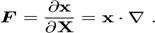
The deformation gradient is given by
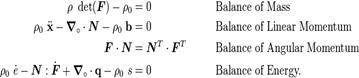
Balance Laws
The operators in the above equations are defined
as such that 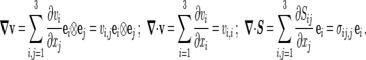
where  is a vector
field, is a vector
field,  is a second-order tensor field, and is a second-order tensor field, and  are the components of an orthonormal
basis in the current configuration. Also, are the components of an orthonormal
basis in the current configuration. Also,
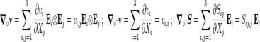
where is a vector
field, is a second-order tensor field, and  are the components of an orthonormal
basis in the reference configuration.
The inner product is defined as are the components of an orthonormal
basis in the reference configuration.
The inner product is defined as
The ClausiusDuhem inequality
http://en.wikipedia.org/wiki/Continuum_mechanics
Summary
These
three media - time, space and energy create sophisticated regional vortex
wave-quantum creation which has beginning and end but by energetic space
time [quantum time genes] create endless recrudescent [evolution]
quantum future continuum time]: with four-dimensional
continuum with four coordinates, the three dimensions of space and that of
time, in which any event can be located mainly by continuum endless evolution
of quantum creation.
This paper may be subject to copy,
but please cited the source.
© Copyright:
Dr. Tejman Chaim, Henry. November 2009
Theory of everything.
http://www.grandunifiedtheory.org.il/
http://en.wikipedia.org/wiki/Chaim_Tejman
|